Constraints and Interactions
Constraints and interactions control how parts in your assembly relate to each other. Choosing the right one affects both how loads are transmitted and how the solver handles degrees of freedom.
What types of interactions are available/ are we going to use?
1. Tie Constraint
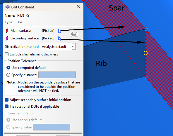
A tie constraint bonds two surfaces permanently — nodes on the slave surface are forced to follow the master with no relative motion. Most common for connecting parts with incompatible meshes.
- Use when: parts are permanently bonded (adhesive joints, welds, skin-to-spar connections)
- Mesh does not need to match at the interface
- No sliding or separation allowed
How to create:
- Go to Constraint → Create
- Select Tie
- Define the master and slave surfaces
- Click OK
2. Rigid Body Constraint
Forces a set of nodes to move as a single rigid object controlled by a Reference Point (RP). The constrained region is treated as infinitely stiff — instead of solving every node independently, Abaqus only tracks the RP.
- Use when: applying a load or BC to a distributed region through a single control point
- No deformation occurs within the constrained region
How to create:
- Go to Constraint → Create
- Select Rigid Body
- Select the region (faces, cells, or node sets)
- Select or create a Reference Point
- Click OK
To load the region: in the Load Module, create a concentrated force or moment and select the RP as the target.
3. Coupling Constraint
Links a reference point to a surface with control over which DOFs are coupled. Two types:
Kinematic — all selected DOFs on the surface nodes are rigidly tied to the RP. Similar to a rigid body but you choose which DOFs are constrained.
Distributing — load is spread from the RP to surface nodes by weighted average. The surface can still deform.
- Use kinematic when you want rigid behavior but need some DOFs free
- Use distributing when you want to apply a resultant load while allowing surface flexibility
4. MPC (Multi-Point Constraint)
User-defined equations relating the displacement of one node to another. Most flexible, most complex. Common built-in types:
- PIN — ties translational DOFs only, no rotational coupling
- BEAM — ties all translational and rotational DOFs
- TIE — ties all DOFs (node-level equivalent of a tie constraint)
5. Shell-to-Solid Coupling
Bridges a shell edge to a solid face, matching both translational and rotational DOFs across incompatible element types. Required when transitioning between shell and solid regions in the same model.
What's the difference between Surface and Node Region for the slave side of a Tie Constraint in Abaqus, and which should I use?
Surface
Defines the slave side using element-based geometry. Abaqus automatically identifies nodes from element faces, respects shell thickness offsets, and projects nodes onto the master surface with tolerance checking.
Node Region
Defines the slave side using a raw node set. No geometric awareness, no shell offset, no projection logic — just explicit node-to-master matching.
Which to Use
Use Surface in almost every case — it's robust, mesh-aware, and handles edge cases automatically.
Use Node Region only when: - Working with an orphan mesh where element-based surfaces can't be defined - Constraining a specific subset of nodes that don't map to a complete element face - Tying embedded reinforcement nodes to a host continuum
Rule of thumb: If you can define a surface, use it. Node Region is a workaround for cases where you can't.
How do I define contact between parts?
Contact is defined in the Interactions Module and requires two steps.
Step 1 — Define the contact property:
- Go to the Interactions Module
- Click Interaction > Property > Create and select Contact
- Click Mechanical and add Tangential Behavior
- Choose the Lagrange friction formulation and enter the coefficient of friction
Step 2 — Define the surfaces:
- Click Interaction > Create and choose Surface-to-Surface Contact
- Define the Master Surface and the Slave Surface
- Master surface nodes can penetrate the slave surface; slave nodes cannot penetrate the master
- Choose the stiffer or coarser-meshed surface as the master
- Select the sliding formulation:
- Finite sliding — allows arbitrary separation, sliding, and rotation (most general)
- Small sliding — limits contact to a small portion of the master surface; requires NLGEOM to be enabled
For most 3D structural models, small sliding is the standard choice.
How does a rigid body simplify the problem?
Without a rigid body, applying a resultant load to a face means either applying individual nodal loads (tedious and mesh-dependent) or using a distributed load with a complex magnitude expression. A rigid body solves this cleanly:
- The entire face is grouped into one rigid set
- A single RP represents the group
- Forces and moments are applied to the RP — Abaqus handles the distribution internally
- Reaction forces and moments at the RP are easy to extract
The trade-off is that the constrained region cannot deform. For load introduction zones where you expect the real structure to flex, consider distributing coupling instead.